Simulating Modular Acoustic Systems

       Given a complex, heterogeneous acoustic system, but absent a closed-form analytic solution to the acoustic wave equation governing its behavior, two natural approaches to modeling it arise: analyze, or decompose the system into smaller modules, or components (for which closed-form analytic solutions to the corresponding wave equations may, or may not, exist); or approximate those solutions numerically that cannot otherwise be solved.

       Modular and numerical approaches are themselves naturally synergistic, as numerical approaches work essentially locally (in time or space), and modular setups provide the 'locales', or distributed elements on which numerical simulation can then be carried out. An example of a mathematical and corresponding computational model for a modular framework which leverages numerical methods is presented in [1]. It is a model of acoustic wave propagation for a class of systems comprised of distributed instances of canonical elements of bar and plate type, which are connected using instances of an auxiliary coupling type interaction. The continuous mathematical description is presented in a corresponding discrete form by way of time domain finite difference approximations to the corresponding exact partial differential equations governing acoustic wave propagation. The model is parametric in the set of the acoustic objects, as well as the set of coupling interactions which connect them.

       The following documents mainly the results of my attempt to implement a simplified version of the model in [1], as well as contains certain remarks which have followed from contemplation of the general role of such models, what it seems historically to have been, and would seem poised going forward to be in the field of computational acoustics.

       It contains: (1) a summary of the model in [1]; (2) a simplified version, with discretization, of the model in [1]; (3) an overview of a corresponding C++ implementation of the simplified model; (4) a demonstration of some audio and visual examples generated using the implementation; (5) some remarks on possible generalizations and directions for future work.

Part 1. Mathematical Model

The mathematical model for continuous vibration of a single plate (I’ll exclusively treat plates in what follows) presented in [1] is the following equation:

Here, \(u_{x,y,t}\) represents transverse displacement of the plate; \(\kappa\) is a parameter controlling the plate stiffness, the terms with coefficients \(\sigma_{0}\) and \(\sigma_{1}\) correspond, respectively, to frequency independent, and dependent decay, and the summation is taken over a set q of couplings or external excitations, each of which is localized by a corresponding Dirac delta-type distribution, \(E_{q}\). The operators \(\Delta\) and \(\Delta^2 = \Delta \cdot \Delta\) are the Laplacian and its square, the Biharmonic operator or Bilaplacian, discussion of which both will be deferred until later.

Dirichlet (clamped) boundary conditions of the form

are exclusively treated in what follows, but pivoting (Neumann), free, mixed, etc. boundary condition types are also possible.

Connections are encoded as pairs of coupled differential equations, of the form:

In [1], \(F_{c}\) and \({F}_{c}^{*}\) are related by a nonlinear spring type interaction,

where \(M_{(1/2)}\) is a constant representing the mass ratio of the two plates. Such a choice of connection element is perhaps attractive for being simple enough to have a tractable semi-implicit solution, yet still nonlinear and so potentially producing of interesting dynamics, and perhaps most importantly, it exhibits a symmetry which will lead to a quantity of the system being conserved.

(However, \(F\) and \(F^*\) need, in principle, not be related symmetrically, nonlinearly, or in any particular way. In the simplified model below, we will take the approach that the flow of interaction across a coupling is directed, and model it simply as a sum of acoustic potential or velocity over the region of contact. Symmetric connections are then recovered as pairs of directed ones.)

A complete system is then comprised of an indexed set of instances of plates and connections between them, where at each time \(t\) inputs flow to the plates from excitations or coupling interactions, and the plates then evolve according to the above equations. The output of the system is then given by the collection of height fields representing transverse displacements, and can be sampled as:

where the brackets indicate an \(L^2\) inner product. Output may then feed back, through the couplings, into the system as input.

Part 2. Simplified Model and Discrete Formulation

I consider the following simplified form of the above equation for plate vibration:

with simplified directed connections:

where

and

is the inner product of the height field \(u\) with the localizing distribution \(E_{c}\).

It is an augmented inhomogeneous acoustic wave equation, in the sense that it combines contributions from the Laplacian and at least one of its powers, as well as a sum of forcing terms, which arise from the simplified, directed (non-conservative) couplings:

This continuous-time model can be discreted using finite differences as follows. A common approximation to the Laplacian, used in [1], is::

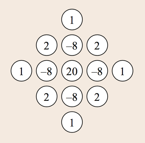
Where \(h\) is the grid spacing. Applying this formula for all points in the domain corresponds to convolving the function \(u\) with the well-known 5-point stencil. A similar formula for the Bilaplacian, which aggregates values from two rings of neighbors around the central point, is given by convolution with the following 13-point stencil:

Finally, an approximation to the first temporal derivative is given by the backward difference operator:

where \(k\) is the sample period, or time-step (and so \(\frac{1}{k}\) the sampling rate).

Part 3. Overview of Implementation

(Note: I developed the C++ implementation for this project prioritizing speed; consequently, I eschewed certain good-practices, such as keeping member variables private or accessible only by getters and setters.)

The above simplified and discrete model was implemented in C++ using a small set of C++ classes and structures. The essential class was Surface, whose .hpp file looked like this:

Surface.hpp

class Surface{
    
    glm::vec3 basepoint;
    glm::vec3 normal;
    double scale;
    
    int side_length;
    int divisions;
    
    std::vector<GLfloat> vertsNormalsAndHeights;
    
    double biharm_coeff;
    double lap_coeff;
    
    unsigned long int reset_heights_counter;
    
    double wave_speed;
    double dampening;
    
    std::deque<float> output_buffer; //buffer to output file
    
public:
    
    Surface(glm::vec3 basepoint, glm::vec3 normal, double scale, int sideLen, int divs, double biharm_coeff, double damp, double wave_sp);
    
    std::vector<std::vector<Vertex>> vertices;
    std::vector<VResonator> vresonators;
    
    void create();
    void draw();
    void beginUpdate();
    void endUpdate();
    
    glm::vec3 getBasepoint();
    glm::vec3 getNormal();
    void setBasepoint(glm::vec3 bpoint);
    void setNormal(glm::vec3 norm);
    void update_vresonators();
    
    void initialize();
    void recalibrate_heights();
    void compute_laplace();
    void compute_biharmonic();
    void evolve_boundary();
    void evolve_interior();
    void evolve();
    void sample_output();
    
    std::vector<GLfloat>* getVertsNormalsAndHeights();
    void write_output(std::string name);    
};

Each surface is simply a square, whose basepoint and global normal vector situate it in \({\mathfrak{R}^3}\). It contains a C++ vector of Vertices, which are very simple structures designed simply to store the all of the values (heights, spatial and temporal first and second derivatives) defined over the Surface; the vertices are indexed by Cartesian coordinates over the surface, so in aggregate they store matrices of each of the above different types of values.

The core of the methods implemented in Surface.cpp (i.e., excluding methods related, e.g., to preparing vertices for rendering in OpenGl) are the following:

Surface.cpp methods

void Surface::beginUpdate(){
    for(int i = 0; i < side_length; i++){
        for(int j = 0; j < side_length; j++){
            Vertex* v = &(vertices[i][j]);
            v->l_vals[0] = v->getHeight();
        }
    }
}



void Surface::endUpdate(){
    for(int i = 0; i < side_length; i++){
        for(int j = 0; j < side_length; j++){
            Vertex* v = &(vertices[i][j]);
            v->setHeight(v->l_vals[0]);
        }
    }
}

void Surface::update_vresonators(){
    for(int i = 0; i < vresonators.size(); i++){
        VResonator* vr = &(vresonators[i]);
        vr->updateVResonator();
        Vertex* v = &vertices[vr->getX()][vr->getZ()];
        v->l_vals[1] += vr->gettVelocity() * waveSpeed;
    }
}

void Surface::compute_laplace(){
    for(int i = 1; i < side_length - 1; i++){
        for(int j = 1; j < side_length - 1; j++){
            Vertex* vc = &(vertices[i][j]);
            Vertex* vr = &(vertices[i+1][j]);
            Vertex* vl = &(vertices[i-1][j]);
            Vertex* vu = &(vertices[i][j+1]);
            Vertex* vd = &(vertices[i][j-1]);

            double laplace = (vl->l_vals[0] + vr->l_vals[0] + vd->l_vals[0] + vu->l_vals[0] - 4.0 * vc->l_vals[0]);
            double height = ((2.0 * vc->l_vals[1]) - vc->l_vals[2] + (pow((swave_speed), 2.0) * laplace * dampening));
            vc->temp_vals[0] = height;
        }
    }
}

void Surface::compute_biharmonic(){
    
    double mu = 0.25; //1.0/side_length;
    double mu2 = mu * mu;
    
    for(int i = 2; i < side_length - 2; i++){
        for(int j = 2; j < side_length - 2; j++){
            
            Vertex* vc = &(vertices[i][j]);
            Vertex* vr = &(vertices[i+1][j]);
            Vertex* vl = &(vertices[i-1][j]);
            Vertex* vu = &(vertices[i][j+1]);
            Vertex* vd = &(vertices[i][j-1]);
            Vertex* vru = &(vertices[i+1][j+1]);
            Vertex* vlu = &(vertices[i-1][j+1]);
            Vertex* vrd = &(vertices[i+1][j-1]);
            Vertex* vld = &(vertices[i-1][j-1]);
            Vertex* vrr = &(vertices[i+2][j]);
            Vertex* vll = &(vertices[i-2][j]);
            Vertex* vuu = &(vertices[i][j+2]);
            Vertex* vdd = &(vertices[i][j-2]);
            
            
            double height = (2.0 * vc->l_vals[1]) - 20.0 * mu2 * vc->l_vals[1] + 8.0 * mu2 * (vr->l_vals[1] + vl->l_vals[1] + vu->l_vals[1] + vd->l_vals[1]) - 2.0 * mu2 * (vru->l_vals[1] + vlu->l_vals[1] + vld->l_vals[1] + vrd->l_vals[1]) - mu2 * (vrr->l_vals[1] + vll->l_vals[1] + vuu->l_vals[1] + vdd->l_vals[1]) - vc->l_vals[2];

            vc->bi_vals[0] = height;
        }
    }
}


// boundary evolve
void Surface::evolve_boundary(){
    for(int i = 0; i < side_length; i++){
        
        Vertex* vr = &(vertices[side_length - 1][i]);
        Vertex* vl = &(vertices[0][i]);
        Vertex* vt = &(vertices[i][side_length - 1]);
        Vertex* vb = &(vertices[i][0]);
        
        vr->l_vals[1] = vr->l_vals[0];
        vr->l_vals[0] = vr->temp_vals[0];
        
        vl->l_vals[1] = vl->l_vals[0];
        vl->l_vals[0] = vl->temp_vals[0];
        
        vt->l_vals[1] = vt->l_vals[0];
        vt->l_vals[0] = vt->temp_vals[0];
        
        vb->l_vals[1] = vb->l_vals[0];
        vb->l_vals[0] = vb->temp_vals[0];
    }
}

void Surface::evolve_interior(){
    for(int j = 1; j < side_length - 1; j++){
        for(int k = 1; k < side_length - 1; k++){
            
            Vertex* v = &(vertices[j][k]);
           
            if(sbiharm_coeff >= .99){
                v->l_vals[0] = v->bi_vals[0];
            }
            else if (sbiharm_coeff > .01)
                v->l_vals[0] = sbiharm_coeff * v->bi_vals[0] + (1.0 - sbiharm_coeff) * v->temp_vals[0];
            else if (sbiharm_coeff <= 0.1){ // only laplacian
                v->l_vals[0] = v->temp_vals[0];
            }
            
            v->l_vals[2] = v->l_vals[1];
            v->l_vals[1] = v->l_vals[0];
        }
    }
}

void Surface::evolve(){
    
    if(sbiharm_coeff >= .99){
        compute_biharmonic();
    }
    else if (sbiharm_coeff > 0.1){
        compute_laplace();
        compute_biharmonic();
    }
    else
        compute_laplace();
    
    evolve_boundary();
    evolve_interior();   
}

void Surface::sample_output(){
    int coord = side_length / 2 - 2;
    output_buffer.push_front(vertices[coord][coord].l_vals[0]);
    if(output_buffer.size() > sample_rate * 120){
        output_buffer.pop_back();
    }
}

void Surface::write_output(std::string name){
    writeWav(&output_buffer, name.c_str());
}

I won’t expound what’s going on above, beyond merely mention that perhaps the subtlest aspect of the above evolution algorithm is getting the order of operations (see the function evolve()) right. If you update values in the wrong order, you may get numerical chaos, or zero response from the system.

The coupling structure is comparatively simple; it simply indexes a pair of surfaces, and identifies points where the interaction is to take place:

Coupling.hpp

struct coupling{
    unsigned int s1_id, s2_id; // indices of coupled surfaces
    int s1_x, s1_z, s2_x, s2_z; // coordinates of coupling points
    double amplification;
    
    coupling(unsigned int id1, unsigned int id2, int x1, int z1, int x2, int z2, double amp)
    {
        this->s1_id = id1; this->s2_id = id2; this->s1_x = x1; this->s1_z = z1; this->s2_x = x2; this->s2_z = z2; this->amplification = amp;
    }
};

Everything is then tied together in Main, where graphics run in a separate thread to the audio and numerical simulation. On a 2-core, 2015 Macbook Pro, with three Surfaces of sizes 100x100, 80x80, and 60x60 (see GIF) and three couplings, the system audio rate was between 3-400 fps.

Part 4. Examples

Below is an example of a modular system that was simulated using the implementation. The graphics appear fine at 60 Hz, but for the audio, a sample rate of 3-400 Hz is barely enough to resolve any frequency above the lower limit of what is audible to human hearing. In an attempt to reveal some information about the system through its audio output, I’ve sped-up the audio samples which follow – which were sampled from the centers of the middle, and bottom plates, respectively, and were initially ~two minutes long each – by a factor of 60 and looped them a few times. The result is low rumbles, each somehow a (very noisy) filter of the input signal coming from the top plate, which is evolving by the Bilaplacian.

The expense of numerically simulating 2- and higher dimensional wave equations unfortunately precludes one from obtaining sound results of any interest, if one is running their experiments, as I did, on standard hardware like a phone or laptop in 2020. However, as demonstrated by the investigations documented in [2], and by the NESS Project [3], real-time simulation of 2- and 3- dimensional acoustic systems is possible using parallelization and hardware acceleration. In fact, the statement that such real-time results are possible is banal on a conceptual level, since the actions of the operators involved in the wave equations are all local and ‘embarrassingly-parallel’. I.e., improvement in the execution time of an algorithm to compute acoustic wave equations, of the form described above, by addition of further processing units will increase essentially linearly, according to Amdahl’s Law. However, constructing actual examples of such real-time systems, in practice, is another matter.

Part 5. Closing Remarks: Generalizations and Future Work

The power of a modular approach such as the one in [1] comes from its ability to decompose certain complex systems into, or synthesize them from, sets of canonical elements for which localized solutions to governing equations exist, and are tractable. For any such modeling framework, the class of complex systems that can be approximately analyzed or synthesized within the framework will depend upon the set of canonical elements, and different ways of connecting, or composing instances of those elements together. For the model in [1], the class of approximable systems corresponds precisely to all combinations of rectangular plates (and bars) connected via the defined type of coupling interaction. Such a characterization of the space of models possible within a given modular framework then raises the obvious question - by generalizing or refining the set of canonical elements and couplings, can the space of approximable systems within the framework correspondingly be expanded or refined?

In the case of the model from [1], perhaps the most obvious such approach to varying the underlying set of elements is to replace the notion of bar and plate with the more general mathematical one of manifold – a shape which looks essentially the same, locally, everywhere – or hypersurface (manifold of dimension \(N-1\) embedded in an ambient space of dimension \(N\)). Substituting such a more general notion of shape then correspondingly requires providing a modified scheme for numerically simulating acoustic wave propagation over the domain which that shape parameterizes. In the case of at least a surface (understood as a manifold) which admits a triangulation, this can be achieved by replacing the expression of the Laplacian given in Cartesian coordinates with a more general formulation (see [6] for details), known as the Cotangent Laplacian:

where the \(u_{j}\) are neighbors of the central vertex \(u_{i}\):

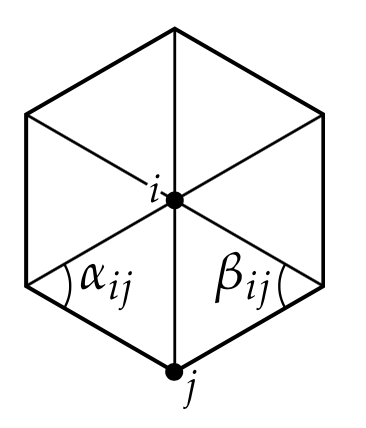
Further generalizations are certainly possible - for example, to situations in which the underlying geometry is not static, but dynamic, and somehow coupled, itself, to the functions which are defined upon it. This is the case, e.g., in so-called adaptive finite element methods, and can be instrumental in minimizing noise due to, e.g., anistropy.

Lastly, the corresponding notion of connection between elements also must be changed once that of the underlying elements is, and when the prototypical notion of shape becomes that of a manifold, that of connection must be adapted somehow to involve the notion of a map or attachment between manifolds.

References

[1] A Modular Percussion Synthesis Environment; Bilbao (2009)
[2] On the Limits of Real-Time Physical Modeling Synthesis with a Modular Environment; Webb, Bilbao (2015)
[3] NESS Project, https://www.ness.music.ed.ac.uk/archives/systems/modular-environments
[4] Finite Difference Schemes in Musical Acoustics: A Tutorial; Bilbao, Hamilton, Harrison, Torin (2018)
[5] “We’ve had Laplacian, yes. What about Bilaplacian?”; Stein (2020)
[6] Laplace-Beltrami:The Swiss Army Knife of Geometry Processing; Crane, Solomon, Vouga (2014)